Choice Part 1

Today’s post is about consumer choice. Previously we have looked at the indifference curve and the budget line. We will now use these two concepts together to determine what the optimal choice is for the consumer.

For almost all combinations of budget lines and indifference curves, the optimal choice for the consumer will be the point at which the budget line is tangent to the indifference curve. This is the point where the entire budget is being spent in order to achieve the greatest level of utility. The fact that the indifference curve needs to be tangent is important. If it crossed the budget line, this would mean that there is some point on the budget line that is above the indifference curve. In essence there would be a more optimal bundle that would give greater utility and that the consumer would be able to afford.

There are some exceptions to this. The first is if the indifference curve has a kink at the optimal choice. In this case the tangent just isn’t defined. This case however does not have much economic significance. The second exception is when the optimal point occurs where the consumer of some good is zero. In other words where the consumer is only consumer one good. This is what we call a boundary optimum.

So if we assume that the consumer is consuming some of both goods and if we assume that it is not kinked than tangency is a necessary condition for optimal choice. Just because it is a necessary condition though, does not mean that it is a sufficient condition. There are some cases however when it is sufficient, and this is the case of convex preferences. In the case of strictly convex preferences, any point that satisfies the tangency condition must be an optimal point. It can also be the case that there is more than one optimal point.

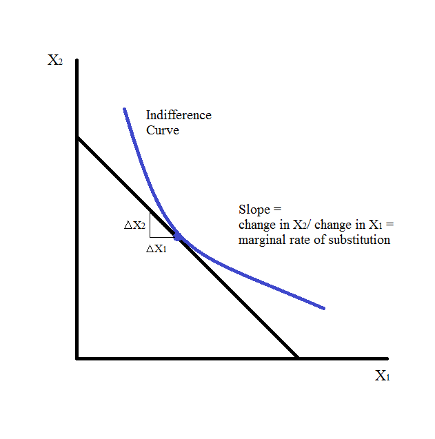
As we have said before, MRS (marginal rate of substitution) must equal the slope of the budget line at an interior optimum. What does this actually mean economically though? One of our interpretations of the MRS is that is the rate of exchange at which the consumer is just willing to stay put. This means that if the MRS is different from the price ratio then there is an exchange that the consumer will be willing to make and that they cannot be at their optimal choice.

While this is short choice is a pretty complicated topic and I will try to spend quite a bit of time on it, in order to try and explain it as well as using the time to understand it myself.

Utility Part 2

Todays post will be a continuation of the discussion about utility. Last time we left off with a talk about perfect complements. Today we will start with quasilinear preferences.

Quasilinear preferences are a shape of indifference curve that we haven’t looked at yet. A consumer has indifference curves that are all just vertically shifted versions of one indifference curve. The equation for an indifference curve will take the form x₂ = k – v(x₁) where k is a difference constant for each indifference curve. This equation says that the height of each indifference curve is some function of x₁, -v(x₁), plus a constant k. Higher values of k give higher indifference curves.

The natural way to label indifference curves here is with k – roughly speaking, the height of the indifference curve along the vertical axis. Solving for k and setting it equal to utility, we have:

 u(x₁, x₂) = k = v(x₁) + x₂

In this case the utility function is linear in good 2, but (possibly) nonlinear in good 1; hence the name quasilinear utility, meaning partly linear utility. Quasilinear utility functions are not particularly realistic, but they are very easy to work with.

Another commonly used utility function is the Cobb-Douglas utility function. It takes the form:

U(x₁, x₂) = x₁^cx₂^d

Where c and d are positive numbers that describe the preferences of the consumer. Cobb-Douglas indifference curves look just like the nice convex monotonic indifference curves that we referred to as well behaved indifference curves in a previous post. Cobb-Douglas are the standard example of indifference curves that look well-behaved, and in fact, the formula describing them is about the simplest algebraic expression that generates well behaved preferences.

If we consider a consumer with some bundle of goods (x₁,x₂) we may want to know how their utility changes if we give them a little more of good 1. This rate of change is called the marginal utility with respect to good 1. We write it as MU₁ and think of it as being a ratio.

MU₁ = ΔU/Δx₁ = [u(x₁ + Δx₁, x₂) – u(x₁, x₂)]/Δx₁

It measures the rate of change in utility (ΔU) associated with a small change in the amount of good 1 (Δx₁). Note that the amount of good 2 is held fixed in this calculation.

This definition implies that to calculate the change in utility associated with a small change in consumption of good 1, we can just multiply the change in consumption by the marginal utility of the good:

ΔU = MU₁Δx₁

The marginal utility with respect to x₂ is defined in a similar manner. It is important to realize that the magnitude of marginal utility depends on the magnitude of utility. Thus it depends on the particular way that we choose to measure utility. If we multiply utility by 2, then marginal utility would also be multiplied by 2. We would still have a perfectly valid utility function in that it would represent the same preferences, but it would just be scaled differently.

This means that marginal utility itself has no behavioral content. How can we calculate marginal utility from a consumer’s choice behavior? We can’t. Choice behavior only reveals information about the way a consumer ranks different bundles of goods. Marginal utility depends on the particular utility function that we use to reflect the preference ordering and its magnitude has no particular significance. However it turns out that marginal utility can be used to calculate something that does have behavioral content.

A utility function can be used to measure the marginal rate of substitution (MRS). Recall that the MRS measure the slope of the indifference curve at a given bundle of goods; it can be interpreted as the rate at which a consumer is just willing to substitute a small amount of good 2 for good 1.

This interpretation gives a simple way to calculate the MRS. Consider a change in consumption of each good, (Δx₁, Δx₂), that keeps utility constant – that is, a change in consumption that moves us along the indifference curve. Then we must have

MU₁Δx₁ + MU₂ Δx₂ = ΔU = 0

Solving for the slope of the indifference curve we have

MRS = Δx₂/ Δx₁ = -MU₁/MU₂

The algebraic sign of the MRS is negative: if you get more of good 1 you have to get less of good 2 in order to keep the same level of utility. However it gets very tedious to keep track of the minus sign, so economists often refer to the MRS by its absolute value – that is, as a positive number.

This is a continuation of utility as I talked about last week. Tomorrow I will be looking at the next chapter which is on choice.

Habits

I have just finished reading, The Power of Habit by Charles Duhigg. I know that this is not about economics but today I am just going to talk a bit about what I read and why I think it is important and how it relates to my goals for this blog.

To start off with, I highly recommend this book. It was recommended to me and actually given to me. Even with this though it took me around 6 months before I started reading it. The book is very clearly laid out and a very interesting, if at times disturbing, read. For example it talk about how companies are able to use information on us to gain insight into our habits and market stuff to us specifically. While this is probably no surprise at all to anyone who uses the internet, the amount of information and just how accurate they can be, is something that to me at least I found a bit surprising. The real point of this book though is that habits can be changed and he gives steps and examples of how you can go about changing them.

For me personally, there are some habits that I would like to get rid of as well as some habits that I would like to gain. Such as an increase in my amount of exercise. Exercise is something that I have struggled with since graduating high school. As well studying and procrastination has always been a big problem, something that I talked about at the beginning of this blog. While I think that this has done some good, I have also been struggling a lot with regularly studying and writing in this blog. Reading about habits has helped me in some ways to understand where to start from in terms of changing my behaviour to something that I will be happier with in my own life.

I think that having bad habits can sometimes be very frustrating. Habits are hard to control and having habits that we don’t want or would like to change can leave us feeling like we don’t have much control over our lives. At least I personally know that I feel that way sometimes. In the book Duhigg talks about how belief is one of the most important parts of changing habits. In order for us to be able to change our habits we need to believe that they can change. I know that this is a very hard thing for me, as I tend to be a pretty skeptical person about most things and at the same time, like most people from my generation probably, I crave immediate results. However, knowing that I can do something in a concrete way, might help me to find the belief that I need in order to change my behaviour.

I have often found that I reward myself through food and this is one of the major things that I feel I want to change. I have really struggled with finding other rewards that work for myself though and I think that will be one of the hardest parts of changing. Probably where I will start is where Duhigg recommends, which is to identify the routine. I need to find a routine that I do that that I would like to change. In an effort to do this I think I will start trying to write down more of what I do in a given day to see what habits I actually have. As well I need to figure out why food is such a good reward for me. This will help me figure out what exactly I crave in a reward and hopefully figure out a way to choose a different reward that gives me the same pleasure but that I am happier with myself.

I will leave with just a short piece on economics. One of the core components to Duhiggs book is on the behaviour on businesses and consumers, both of which are governed by habits. I think habits are something that would be very interesting to do a more in depth study of in terms of economic behaviour as we may find that it explains a lot of the behaviour that economists can often find puzzling. This is a book that I feel will have a big impact on my life and once again I highly recommend taking a look at it for yourself.

EconTalk Fair Trade vs Free Trade

Today’s blog I will talk about another EconTalk. This was supposed to have been yesterday’s blog but because of various circumstances I was not able to post yesterday. The EconTalk that I listened to was on fair trade and free trade. The guest on the show was Amrita Narlikar. The talk can be found here http://www.econtalk.org/archives/2013/07/narlikar_on_fai.html.

This was a very interesting EconTalk. Narlikar wrote an article that you can find here about fair trade practices http://www.foreignaffairs.com/articles/139127/amrita-narlikar-and-dan-kim/unfair-trade. The basic premise behind the arguments from Narlikar is that fair trade is not necessarily as good for producers as it is said to be. She looks at the impact on non-fair trade farmers in the same area and how fair trade could hurt the domestic market where fair trade goods are produced. Her logic for this is based around a couple of things.

The first is that because fair trade goods receive a premium, farmers are more likely to try and grow those goods. However most fair trade goods are things like coffee and tea. This leads farmers away from growing crops that they might use to feed themselves. Another one of the ideas is that since fair trade goods only receive a premium when they are sold internationally that makes farmers not want to sell their product domestically, hurting the domestic market. Finally she looks at the problem of fair trade certification being expensive for farmers to obtain.

All of these are interesting points but there did not seem to be a huge amount of evidence that this is the reality of the situation. Narlikar argues that true free trade is what would provide a larger benefit for least developed countries. Her arguments for this seems primarily focused around the subsidies and trade barriers that the developed countries put in place. She argued that these should be lessened or gotten rid of so that lesser developed countries will be able to compete better on an international level.

I think that while there are some good aspects to this article there are also a lot of problems as well. In my own, relatively uninformed opinion, there is a huge problem with poorer countries being taken advantage of. While I think that moving towards more free trade will be beneficial in some ways, such as removing subsidies and trade barriers that the richer countries put on the poorer countries that is not usually what happens when so called free trade is actually implemented.

Utility Part 1

Today’s post is about Utility. This will probably be the theme for the next couple of posts because it is a pretty important part of consumer preference economics.

Utility is a bit of a complicated topic. It used to be that when utility was a reference to a person’s overall well-being. It was a numeric measure of a person’s happiness. The problem with this is that it is very difficult to translate happiness into a number depending on choices. As such for the purposes of this brand of economics utility will used only as a way to describe preferences.

For economists all that matters is whether one bundle has a higher utility than another, how much higher really doesn’t matter. A utility function is a way of assigning a number to every possible consumption bundle such that more-preferred bundles get assigned larger numbers than less-preferred bundles. The only property of a utility assignment that is important is how it orders the bundles of goods. Because of the emphasis on ordering bundles of goods, this kind of utility is referred to as ordinal utility.

There are many examples of utility functions. A utility function looks like the following u(x₁, x₂). Depending on what type of goods there are different utility functions exist. For example with perfect substitutes. If we go back to the example of red and blue pencils we can see how this works. In this example all that mattered to the consumer is the number of pencils not whether they were red or blue. In this case the utility function looks like the following u(x₁, x₂) = x₁ + x ₂. To see that this works we can ask two questions. Is this utility function constant along the indifference curve and does it assign a higher label to a more-preferred bundle. The answer to both questions is yes, so we have a utility function.

If the consumer is willing to substitute good 1 for good 2 at a different rate, say 2 to 1 then we end up with a different utility function. It would look like this u(x₁, x₂) = x₁ + 2x₂. This means that the consumer values good 2 twice as much as good 1. The general form for a utility function with perfect substitutes is u(x₁, x₂) = ax₁ + bx₂ where a and b are some positive numbers that measure the value of goods 1 and 2 to the consumer.

Another type of utility function is for perfect complements. This is the case with left and right shoes. When these are the two goods the only thing that the consumer cares about is how many complete pairs of shoes they have. In this case the number of pairs of shoes that they have is the minimum of the number of right shoes you have x₁, and the number of left shoes you have, x₂. Thus the utility function of perfect complements takes the form u(x₁, x₂) = min{x₁, x₂}. If we look at shoes it is pretty easy to see that this holds. If we have 5 right shoes and 5 left shoes than the function would be u(x₁, x₂) = min{5,5} and so the utility would be five. If we increase the number of left shoes the utility should stay the same and we can test this. If we now have 5 right shoes and 7 left shoes our utility function would be u(x₁, x₂) = min{5,7} which equals 5. We can see here than that the function works.

The same way that we were able to change the one to one ratio of perfect substitutes also works here. As such the general formula for perfect complements is u(x₁, x₂) = min{ax₁, bx₂}. Where a and b are positive numbers that indicate the proportions in which goods are consumed.

This is a brief look at utility and some different types of utility functions. There is more to talk about however and so I will be posting more on this later in the week.

Marginal Rate of Substitution

Todays post is on the marginal rate of substitution. This is out of the third chapter of the textbook and is an important component of the indifference curve. The marginal rate of substitution is the slope of an indifference curve.

The name for the MRS comes from the fact that the MRS measures the rate at which the consumer is just willing to substitute one good for the other. If we take some small amount of good 1, Δx₁, away from the consumer. Then we give the consumer Δx₂, an amount that is just sufficient to put him back on his indifference curve, so that he is just as well off after this substitution of x₂ for x₁ as he was before. We think of the ratio Δx₂/Δx₁ as being the rate at which the consumer is willing to substitute good 2 for good 1.

One slightly confusing thing about the MRS is that it is typically a negative number. We’ve already seen that monotonic preferences imply that indifference curves must have a negative slopes. Since the MRS is the numerical measure of the slope of an indifference curve, it will naturally be a negative number.

The marginal rate of substitution measures an interesting aspect of the consumer’s behavior. Suppose that the consumer has well behaved preferences, that is, preferences that are monotonic and convex, and that he is currently consumer some bundle (x₁, x₂). We now offer him a trade: he can exchange good 1 for 2, or good 2 for 1, in any amount at a “rate of exchange” of E.

That is, if the consumer gives up Δx₁ units of good 1, he can get EΔx₁ units of good 2 in exchange. Or, conversely, if he gives up Δx₂ units of good 2, he can get Δx₂/E units of good 1. Geometrically we are offering the consumer an opportunity to move to any point along a line with slope –E that passes through (x₁, x₂), as depicted below.

We can now ask what the rate of exchange would have to be in order for the consumer to want to stay put at (x₁, x₂). To answer this question, we simply note that any time the exchange line crosses the indifference curve, there will be some points on the line that are preferred to (x₁, x₂) – that lie above the indifference curve. Thus if there is to be no movement from (x₁, x₂), the exchange line must be tangent to the indifference curve. That is, the slope of the exchange line, -E must be the slope of the indifference curve at (x₁, x₂). At any other rate of exchange, the exchange line would cut the indifference curve and thus allow the consumer to move to a more preferred point.

Thus the slope of the indifference curve, the MRS, measures the rate at which the consumer is just on the margin of trading or not trading. At any rate of exchange other than the MRS, the consumer would want to trade one good for the other. But if the rate of exchange equals the MRS, the consumer wants to stay put.

The MRS can also sometimes be useful in describing the shape of the indifference curve when we look at its behavior. For example, the perfect substitutes indifference curves are characterized by the fact that the MRS is constant at -1. The neutrals case is characterized by the fact that the MRS is everywhere infinite. The preferences for perfect complements are characterized by the fact that the MRS is either zero or infinity, and nothing in between.

This is a bit about the marginal rate of substitution. It is a very important concept that will be talked about in the future as well.

EconTalk on Aid, Migration and Poverty

Today I listened to a very interesting EconTalk with Michael Clemens from the centre for global development. It was an incredibly interesting conversation that focused on foreign aid and its impact on poverty as well as a lot of other global factors.

One of the most interesting things that I found out from this talk was that when you compare foreign aid and money sent back home by immigrants, the money sent back home privately comes up to about four times that of foreign aid. Clemens has said that while there is a positive benefit from foreign aid it is a very small benefit. A larger benefit comes from immigration.

They also talked a fair bit about the impact that immigration can have on the receiving countries and both the pros and cons of it. Overall this is a very interesting talk on global development and I highly recommend it. The EconTalk can be found here http://www.econtalk.org/archives/2013/07/clemens_on_aid.html

Habits

Today’s post will be quite a bit different from normal. I received a book as a present a while ago called “The Power of Habit” by Charles Duhigg. I have started reading the book as a way to try to analyze my own habits and see what I can do about changing them. Part of the idea of this blog for the summer was to learn better study habits. While this went okay at the beginning I have had a harder and harder time sticking with what I should be doing.

In an effort to change some of my habits I have started reading this book. Duhigg describes habits as having three parts, a cue that initiates the habit, a routine that is what we do, and a reward that is what we get. In learning to change your habits you need to be able to identify these three things about your habits.

Duhigg tells a lot of stories in his book about people who have changed their habits and about just how powerful habits can be. He even relates them to advertising in business and gives examples as to how habits and cravings are used there.

While I am looking to change several of my habits the book recommends starting with just one. He gives the example of a woman who stops smoking and in doing so changes her entire life. This is an example of a keystone habit that can make a big difference.

For myself probably the biggest habit that I have is of procrastination. It is something that affects my entire life, from not getting enough exercise to not getting my schoolwork done. This is something that I really want to work on changing and I think I will try to follow here as I read through the book, the small steps that I am taking towards doing that.

Economic Measures

I decided to do something a little bit different today. After having a conversation about different measures of a counties well-being I decided to do a bit of a discussion of some of them here. These are by no means all of the measures that exist out there merely a sample.

The first to talk about is the one that is most often used, that of GDP. The GDP of a country is the gross domestic product. This is the sum total of everything that is produced inside a country in monetary terms. Closely related to this is the GNP or the gross national product. The GNP is the sum of all of the citizens of a countries production, even if they are not in the country. This is what makes it differ from the GDP.

While both of these are reasonable economic measures of a countries well-being there are several problems that they both share. One of the first problems is that they do not include a lot of work that actually happens in the economy, any black market exchanges and any non-monetary exchanges are not counted. This includes stuff such as house work. Another problem with both of these measures is that while they are reasonable measures of economic well-being of a country they are not a good measure of the well-being of its people. While GDP-per-capita and individuals well-being is positively correlated it does not tell the whole story. GDP also does not say anything about the environmental impact that economic policies can have. Finally it also does not give a good indication of the inequality that there is in a country. While there are many more reasons than just these that there are problems with GDP these are some of the main ones.

Another popular measure used is the Human Development Index. This measure published by the United Nations Development Program is a combination of health, education and income for the population of a country. It has been revised and is now a fairly good measure of the well-being of the people in a country. It can also be adjusted for inequality which helps. Some of the problems with HDI is that it does not give any indication as to the environmental status of a country, it is purely concerned with the well-being of the population. The only time this would come into effect is if it started to affect one of the three indices.

A measure that has been developed to more accurately view the environmental aspect of economic development is call Green Gross Domestic Product or Green GDP. Green GDP is an attempt to factor in the environmental consequences of economic growth into conventional GDP. It monetizes the loss of biodiversity and accounts for costs caused by climate change. While this is a reasonable measure for economic growth factoring the environment, it in itself, is not a good measure for the overall well-being of the population of a country.

This a just a taste of the measures that are out there to look at. There are many more, and the reality is that we need to look at multiple measure to accurately determine the well-being of a country as a whole.

Econ Talk Michael Lind on Libertarianism

Today I listened to an Econtalk. I am still not feeling one hundred percent so until I am I will be posting every day but it might be shorter than usual.

Today’s Econtalk was a discussion on libertarianism. Libertarianism is a political and economic idea that liberty is the highest ideal. They usually support free market ideas and limited government intervention. The conversation was on how there seem to be no countries that have ever had a true libertarian society and how it can be difficult to support it given that it has not really been put into practice.

The second part of the econ talk was about how the basic ideas that are taught in beginner economics courses can make for bad policies. When just these beginning ideas are used instead of the more accurate but more complicated ideas this can have a bad effect on economic policy. Michael Lind wrote a blog about it that can be found here. http://www.salon.com/2013/07/08/how_%E2%80%9Cecon_101%E2%80%9D_is_killing_america/ It is very interesting and I highly recommend reading it.