Consumer Preferences Part 2

Today’s post is on the second part of people’s preferences. This is a continuation of the post the day before yesterday. Yesterday’s post was missed because I was sick but hopefully I am feeling better now and will continue for the rest of the posts this week.

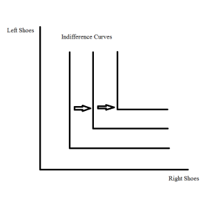
To start off with we will work on perfect complements. Perfect complements are goods that are consumed together in fixed portions. A good example of this is right and left shoes. People like shoes but they always wear left and right shoes together. Having only one shoes instead of both does the consumer no good. The indifference curve for perfect complements looks like this.

If we take a bundle of shoes say (2, 2) the consumer will gain a certain amount of utility from that bundle. Now if we add one more shoe so the bundle is (3, 2) the consumer will be indifferent because they will be no better off than they were before. In fact if the bundle gets changes to (10, 2) or (2, 10) the consumer will still be no better off. The only way they are made better off is when both goods increase at the same rate.

The important thing about perfect complements is that the consumer prefers to consume the goods in fixed proportions, not necessarily that the proportion is one to one.

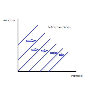
A bad is a commodity that the consumer doesn’t like. An example of this would be if a person like some toppings on a pizza but didn’t like others, such as pepperoni and anchovies. The consumer may like pepperoni but not anchovies, however there may be some amount of pepperoni that would compensate the consumer for having to consume a given amount of anchovies.

First we pick a bundle (x₁, x₂) consisting of some pepperoni and anchovies. If we give the consumer more anchovies, we have to give the consumer more pepperoni to compensate them. Thus the consumer has an indifference curve that slopes up and to the right as in the following.

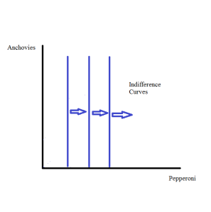
There are also neutral goods.  A neutral good is a good that the consumer doesn’t care about one way or the other. If we take our previous example of the anchovies and pepperoni we can change it so that instead of the anchovies being a bad, instead the consumer is now just neutral towards them. In this case the indifference curve will just be vertical lines. Increasing the amount of anchovies will not take away from the enjoyment of the consumer but neither will it add to it.

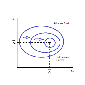
There is also satiation for consumers. This is where there is some overall best bundle for the consumer and the closer they get to that best bundle the better off they are in terms of their own preferences. We assume that the consumer has some most preferred bundle of goods (x-bar₁, x-bar₂), and the further away from the bundle the worse off they are. X-bar is usually written as an x with a line over it, I was unable to find a symbol that works here so I will just write it out as x-bar. In this case we say that (x-bar₁, x-bar₂) is a satiation point and the indifference curve looks like the following.

In this case, the indifference curves have a negative slope when the consumer has too little or too much of both goods and a positive slope when he too much of one good.

There is also the case of discrete goods. For most goods we consume, we think of measuring goods in units where fractional amounts make sense. Over the period of a month you will consumer so many litres of water for example. Sometimes though we want to examine preferences over goods that naturally come in discrete units.

A good example of this is a consumer’s demand for cars. While we could define the demand for cars in terms of the time spent using a car, this would give us a continuous variable. For a lot of people though it is the actually number of cars demanded that is of interest.

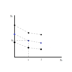
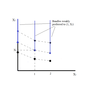
We can use our preference model that we have used previously to describe the behaviour of consumers in this situation the same as we do for anything else. Just like in other circumstances we can use x₁ and x₂. x₁  in this situation would be the discrete good and x₂ will be money, or everything else. The indifference curve for this would look like the following, with the other graph showing the bundles that are weakly preferred.

Usually unless the consumer is consuming only a very small amount of a good, it will be more useful to think about most goods as if they are continuous. As we have looked at several different types of preferences, however it is most useful to focus on a few general shapes of indifference curves. We make some assumptions about these, and with these assumption we call them well-behaved indifference curves.  The assumptions are as follows:

1. We assume monotonicity of preferences. This is basically that we assume more is better. Specifically we are talking about goods and not bads. As we discussed in satiation, there is probably a point where this does not hold, however we will assume that what we are examining are situations before that point is reached.
2. We assume that averages are preferred to extremes.

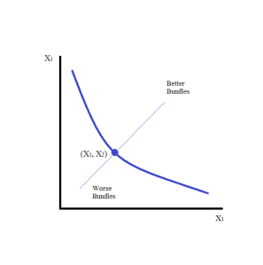
Using these two assumptions most indifference curves will look like the following.

This are some of the basic ideas behind consumer preferences, there is more to come and reality is definitely more complicated than we would like, but this gives us some basic tools to analyze consumer preferences. A key thing to remember is that preferences are generally thought of as over a time period, so our desire for something over a day, a week, or a year. As such this makes them behave differently than if we were just looking at them at a specific time.